Forecasting Movie Box Office Gross Revenue
Movie studios, just as any other commercial enterprise, have limited resources and it is in their interest to be able to accurately estimate the revenue a movie project will generate.
Better gross revenue estimates would assist movie studios in raising funds, creating accurate budgets and optimizing their movie pipeline.
- Data Exploration
- Model Development
- Which Model to Choose?
- Further Work
The Data - Thanks Box Office Mojo!
Using scrapy, I scraped information from Box Office Mojo. I focused on collecting the cumulative weekly total gross revenue for the 100 top grossing movies each year from 1983 to 2017. I also colected each movie’s weekly ranking, genre, duration, rating, budget, and original release data. In all, I downloaded information for almost 1300 movies.
Since the data was collected in json format, I created a script to transform it into a pandas dataframe and a separate one to clean the data and get it ready for analysis.
Examining the Dataset
From looking at the weekly box office for several movies it seemed apparent that most of the revenue for each movie was made in the first few weeks the movie was shown. This led me to speculate that the number of movies premiered in the same week had an impact on the total gross revenue made at the box office, and accordingly I created a new feature to investigate this theory.
Prior to 1999 the dataset has very few movies per year. I decided to only use the movies that started between 1998 and 2016, and whose showing ended by 06/29/2017. That way I am trying to ensure not to include movies that were still being displayed at theaters.

Characteristics of the movies in the Dataset
Using the describe() method in pandas I found out some interesting facts about the movies in the dataset. The average movie duration is aproximately 1 hour 50 minutes with 75% of movies lasting less than 2 hours. The average movie is out in theaters for 15 weeks and 75% of movies are out in theaters 19 weeks. The movie which lasted the longest in theaters was the documentary ‘Deep Sea 3D (IMAX)’ displayed for 580 weeks.
| Duration (HH:MM) | Weeks in Theaters | Gross Box Office (MM) | |
|---|---|---|---|
| 25% | 1:30 | 11 | 40 |
| Mean | 1:50 | 15 | 94 |
| 75% | 2:00 | 19 | 116 |
Distribution of Box Office Gross and Correlations
Inspecting a pair plot revealed the distributions of ‘Box Office Gross’ (‘gtd’ in the plot) and ‘Budget’ to be a bit Log Normal. This led me to used their log values in the regression analysis in order to make their distributions more Normal.

A pair plot of the log of ‘Box Office Gross’ and budget show slightly more normal distributions for these variables.

In our analysis ‘Box Office Gross’ (BGO) is our dependent variable. Examining the correlation of BGO with our other variables we can notice a mild positive (+ve) correlation with movie ‘Duration’ (0.26), stronger +ve correlation to ‘Budget’ and ‘Weeks in Theaters’ (0.6 and 0.45 respectively), and a weak negative (-ve) correlation to number of movies premiering in the same week (-0.12). I decided to drop ‘Weeks in Theaters’ from the analysis, since its seems likely that ‘Weeks in Theaters’ is not known prior to movie release.
Also, budget and movie duration appear mildly +ve correlated (0.33), which alerts me to watch out for evidence of multicollinearity between these variables in our subsequent analysis.
Box Office Gross (BGO) and Budget per year
The mean movie budget seems to have stayed relatively stable at around 50 million, while its distribution seems to be becoming more right skewed with time with the top quartile budgets gradually increasing with time.

BGO distributions are right skewed and the mean budget seems to stay in the 50 to 90 million dollars range through out time.

Movie Premiere conditions
Box Office distribution grouped by number of movies released in a week seem to shift lower as more movies are launched the same week. The mean of the distributions seems to remain in the 10^(7.75) to 10^8 range independently of the number of movies launched in the week.

A release of another movie of the same genre seems to negatively affect Box Office outcomes and shifts its distribution lower.

There does not seem to be a discernable pattern between Box Office Outcomes and day of the week a movie is released, except that the widest range of outcomes seems to occur when movies are released on Fridays.
Developing the Model
Incremental Approach
We are trying to model the log of the Box Office revenue in terms of the particular movie characteristics known prior to the movie premiere.
The initial approach consisted of sistematically adding groupings of features and using sklearn cross validation (5-folds) at each step to verify if the new features increased the explanatory power of the model. We kept in the model those features which increased its explanatory power and did not include those which didn’t.
The steps:
1. Start - Include log of budget - Baseline r2 = 0.16 and MSE = 0.070
2. Add movie duration - both measures deteriorated - Do not include in model.
3. Add number of movies released in the same week - both measures improved - Include in the model.
4. Add the movie studio - both measures deteriorated - Do not include in the model.
5. Add the movie genre - both measures improved - Include in model.
6. Add the movie rating - both measures deteriorated - Do not include in the model.
This procedure led us to a model with 31 parameters which included the log of the budget, the count of movies released the same week, and the genre. The model had an slightly improved r2 of 0.18 and MSE = 0.068.
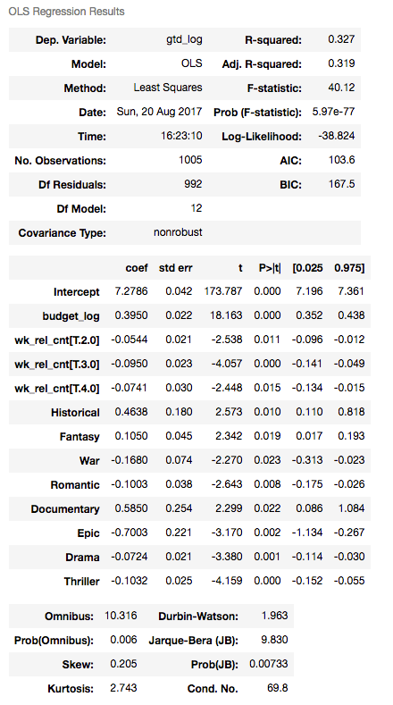
An important step in the development of a linear regression model entails verifying that the model satisfies the linear regression assumptions, including the normality of the residuals and their lack of auto-correlation. I created and fitted an equivalent model using Stats Model OLS() method. To this end, I split my data into a training and test set using a 70/30 split, and fitted my model on the training set.
The model was not great and explained only about 32% of the variation in the data (adjusted r2 = 0.32). Still, the model had an F statistic of 16 with a p-value < 5% further confirming to us that it is highly unlikely this model fitted the data by chance and at least some of the variables included in the model contribute to explain the dependent variable.

A visual inspection tells me the model residuals are centered around the mean.

A Skew of 0.11 and Kurtosis of 2.9 leads me to believe the residuals are normally distributed which is further confirmed by a Jarque-Bera statistic of 2.7 and corresponding p-value of 0.26 (which indicates we cannot reject the null hypothesis of residuals being normally distributed). A Durbin-Watson statistic of 2 tells me there is little evidence the residuals show evidence of auto-correlation.

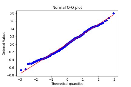
Next I made predictions based on my testing sample set and plotted the residuals against the predictions and a QQ plot of the residuals. The residual plot and the QQ plot seem to indicate the residuals to be slightly right skewed.

One drawback of the above approach is that the order in which the variables are added to the model influences the outcome, as the effect of each added variable on the model is dependent on the variables previously added.
Tuning the Incremental Approach Model
A reasonable simplication to the Incremental Approach model is to drop all those feature coefficients for which their p-values are greater than 0.05 (we cannot reject the hypothesis that these coefficients are different than zero).
Doing this results in a simplified model with 12 features and an slightly lower adjusted r2 than our initial larger model (0.319 Vs. 0.32), and still satisfying our linear regression assumptions of residuals normality and lack of autocorrelation.
Now, maybe we could have achieved similar or more simplified results using regularization.
Using Elastic Net regularization to generate our Model
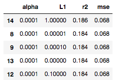
With Elastic Net regularization we need to set the two parameters (alpha and L1) that will penalize our model inclusion of features. To do this effectively I set up a grid to cycle through several combinations of alpha and L1 in a range of values between 1e-5 and 100, created a model for each pair of values, evaluated each model using a 5-fold cross-validation and computed for each model the average r2 and mse across cross-validations.
After doing this the best model (highest average r2 and lowest average mse) was generated with an alpha of 1e-4 and L1 of 1. Its r2 was 0.19 and mse was 0.069.
The resulting model kept 26 features, out of our initial 32.
Using Lasso regularization to generate our Model
I decided to see if a linear model with only Lasso regularization would generate a less complex model (drive the coefficient of more features to zero) so I followed a similar lasso parameter selection procedure as when developing my Elastic Net model, and found out that an L1 value of 1e-4 would produce the highest average r2 and lowest average mse across cross-validations.
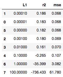
I compared the coefficient values of both the model obtained with Elastic Net regularization against the coefficients obtained using Lasso, and to my surprise, they were equal.
Neither regularization technique was able to simplify the model as much as our Initial Incremental Approach procedure did.

Which model to use?\nRegularized model or Incremental Approach model
The only thing to do was to compare the performance of our Regularized model against or Incremental Approach model, and see if we gain performance by including more features in our model.
I evaluated the performance of the Incremental Approach model using 5 fold cross validation and found that performance was very similar to that of the Regularized models (equal to the second decimal point in both r2 and mse), so until I find evidence that the more complex models would perform better, I would be inclined to choose the Incremental Approach model to reduce complexity.
Further Work
After exhausting the possibilities with our current feature set and still not achieving a satisfactory ‘r2’ and ‘mse’, our next step would be to do some feature engineering and develop new features that can help better explain the variability in the data.
Also, it might be worth investigating if the weekly total domestic gross revenue could be modelled as an exponentially decaying function, estimate its parameters and use this model to estimate total gross domestic revenue.
A big portion of the total gross revenue is made in the first weeks of the movie being shown. Using this information should improve the estimate of the total gross revenue, and could help executives plan for events after premiering the movie like the number of theaters to show the movie, how long to keep the movie on theaters, and how soon to make it available in other media like DVD’s and TV networks.