Human Activity Recognition
My goal is to determine if it is feasible that wearable devices can be used to determine what activities you are doing.
The increase in living standards in our society has brought some mixed blessings. On the one hand, we have abundant food supplies (in some parts of the world), and we tend to live longer, but on the other hand, our sedentary lifestyle has lead to an obesity epidemic and seems linked to sharp decreases in quality of life during our golden years.
With the advent of wearable devices (i.e., Fitbit), the field of human activity recognition (HAR) has gotten a boost. Our hope is that accurate monitoring of human activity will lead us to a better understanding of the link between a sedentary lifestyle and its effects on our health, and also we hope that it should allow us to gently nudge individuals towards a more active lifestyle using by monitoring and positive reinforcement.
Activity identification presents many challenges, one being how to account for the differences in body sizes which leads to individuals displaying different ranges of motion when performing any one activity.
The Dataset
I set out to test if we can use the sensor signals in wearable devices to determine what activity we are performing. To do this, I used a dataset that comprised the data from 18 different activities, performed by nine individuals wearing three inertial devices.
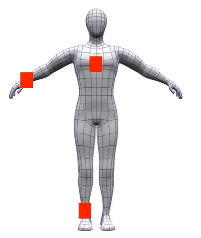
One of the inertial devices was worn on the ankle, another one on the wrist, and another around the chest area.
Information about this dataset can be found in the reference at the end of this article and here: Dataset Source
Preparing the Data
After importing the data, I dropped the features that included individual identifier information and features different from motion or inertia (i.e., subject, heart vari, temperature). I also dropped the information from a second accelerometer in each device that tended to saturate (the range of accelerations detected was too small for some high impact activities such as running), and I also dropped the information from a magnetometer deemed irrelevant by the researchers that collected the data.
Exploring the Data
The data comprised a total of approximately 1.9 million samples distributed across 12 activities and nine subjects.
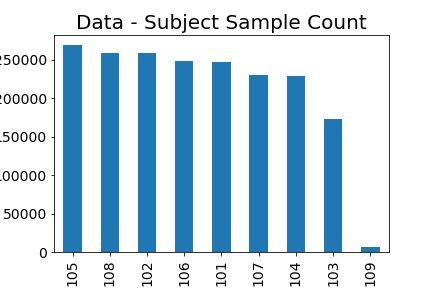
Other than the data for subject 109 with only 7 thousand samples, the data doesn’t seem to present huge imbalances regarding activity or subjects.
The number of sample per activity ranged from 47 thousand (jumping rope) to 230 thousand (ironing), and the number of samples per subject ranged between 170 thousand and 270 thousand samples.

The Process
Establishing a Baseline
Before doing any feature engineering, I wanted to establish a baseline by measuring the average accuracy of three different algorithms using 5-fold stratified cross-validation across the entire dataset using all remaining sensor features.
I did this on three different classifiers: K-Nearest Neighbors (KNN), NaiveBayes (NB), and RandomForest (RF).
I want to see if we could achieve greater than 90% accuracy across each activity, and if so, I wanted to check if could we achieve greater than 90% accuracy with one or two sensors instead of all three.
| Accuracy | f-1 Score | |
|---|---|---|
| KNN | 99 | 99 |
| gaussNB | 75 | 75 |
| RandomForest | 99 | 99 |
I used the scikit-learn default settings when defining the models. KNN uses ten only neighbors by default, and the random forest algorithm depth is automatically determined so that all leaves in the trees contain only one class. This can lead to overfitting, which I suspect is what is happening here with our default KNN and RF classifiers.
Given the poor results obtained by the Naive Bayes classifier, I decided to drop efforts of using it and focus on the KNN and Random Forest classifiers.
To further check the possibility of overfitting the data, I separated my data into a training and test set using a 66/33 split, fitted the classifiers on the training set and evaluated the precision, recall, and f1-score for each class on the test set.
Results for KNN
| class | precision | recall | f1-score |
|---|---|---|---|
| 1 | 1.00 | 1.00 | 1.00 |
| 2 | 1.00 | 1.00 | 1.00 |
| 3 | 1.00 | 1.00 | 1.00 |
| 4 | 0.99 | 1.00 | 0.99 |
| 5 | 1.00 | 1.00 | 1.00 |
| 6 | 1.00 | 1.00 | 1.00 |
| 7 | 0.99 | 0.99 | 0.99 |
| 12 | 1.00 | 0.99 | 1.00 |
| 13 | 1.00 | 0.99 | 1.00 |
| 16 | 1.00 | 1.00 | 1.00 |
| 17 | 1.00 | 1.00 | 1.00 |
| 24 | 1.00 | 1.00 | 1.00 |
| avg/total | 1.00 | 1.00 | 1.00 |
I obtained similar results for my Random Forest classifier. Having 100% precision and recall across all classes increases my suspicions that we are overfitting the training data, and decide to generate learning curves for both classifiers.
Learning Curves
Using features from all sensors, I generated learning curves for my Random Forest classifier where I varied the maximum allowed depth to a value in the range 15 to 35 and did the same for the KNN classifier by varying the number of neighbors to a value in the range 15 to 45.
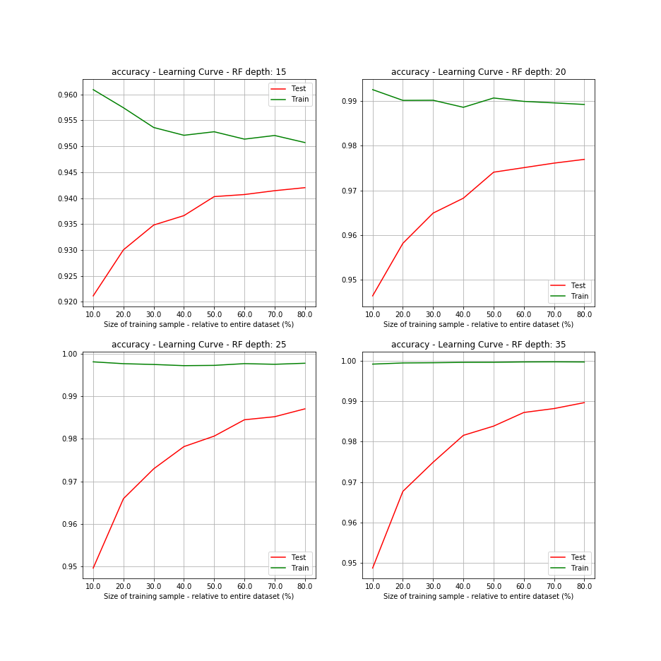
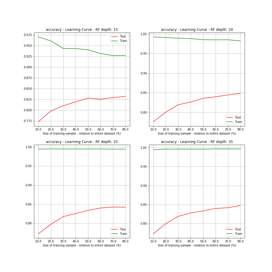
Analyzing the learning curves of the Random Forest classifier we can see that for max tree depths above 15 levels, the accuracy of the classifier on the training data did not decrease when increasing the training sample size confirming my suspicion that the baseline Random Forest classifier was overfitted. As expected we can see that in all cases the accuracy of the classifier on the test data increased as the training sample size increased.
Decreasing our model complexity helped with our overfitting, but as expected came at the expense of reduced accuracy on our test set which now is showing about 94% accuracy when using all of our training data.
Unfortunately, it seems that increasing the size of our training set won’t provide us with much increase in accuracy as the slope of our learning curve seems to be tapering off and converging to its asymptotic values.
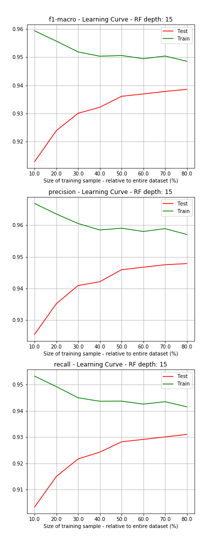
I also checked that the precision, recall and f1 score of the Random Forest classifier with a max depth of 15 also showed behavior consistent with a model that was not overfitting the data and was learning as the size of the training data increased.
What about the learning curve for the K-Neighbors classifier?
On second thought I decided not to generate the learning curves given that the process was very time consuming and I was hitting a deadline. On top of that, it seemed to me that the KNN Classifier code would be bigger than the code for the Random Forest classifier because it has to store the dataset it is trained on to make predictions, which would make it less desirable for wearable devices likely to have memory and processor constraints.
Using One Sensor - Can we achieve high accuracies?
When using all sensors and a random forest with depth 15, we achieved an accuracy of 94% on the test set.
It would be interesting to find out if we could achieve an accuracy greater than 90% using data from only one sensor. Trying to do this makes sense given that a system involving multiple sensors worn on separate parts of the body (separate devices) is more uncomfortable to use, and presents extra technical challenges such as synchronizing the data from the three devices.
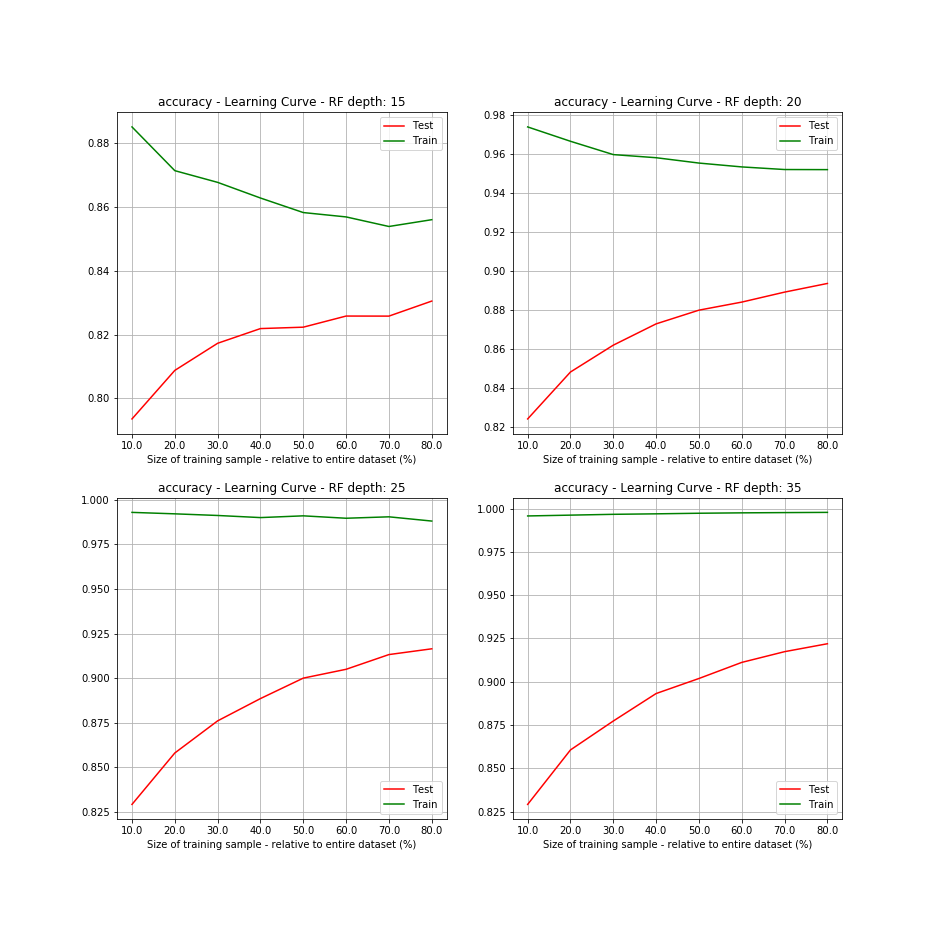
I repeated the previous experiment training our classifiers on only the data from one sensor at a time (ankle, hand, or chest). As before, the classifiers tended to overfit for depths greater than 15. Training the model on data from only one sensor at a time we were able to achieve test data accuracy in the range 82-83%. Below we can see the learning curve for the model being trained only on Hand sensor data.
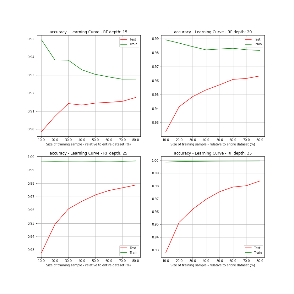
Using two sensors we were able to achieve accuracies between 88% and 91%. Below we can see the learning curve for the model being trained on the Hand and Chest sensor’s data.
Increasing the size of the forest
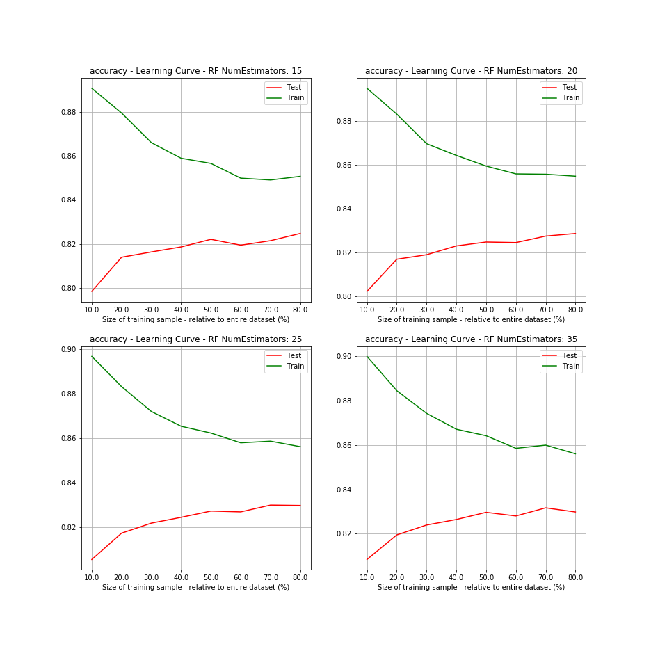
Increasing the number of trees in the Random Forest is an effective way to reduce variance caused by model overfitting, but in our case, the learning curves did not indicate that we were overfitting. I checked anyway if we could increase accuracy by increasing the number of trees in forests of depth 15 but did not achieve an increase in test set accuracy.
Boosting
Boosting is a technique that combines weak learners in such a way to generate an overall strong learner, and has been successfully used in hackathons and Kaggle competitions to achieve increases in accuracy. There are a variety flavors, each with its pros and cons. To start, I decided to run a parameter grid search with 5-fold cross-validation using sklearn’s Gradient Boosting Classifier (GBC). I decided to focus on using data from the hand sensor given that individuals already wear wrist devices (watch) and it wouldn’t be hard to incorporate an extra sensor in the electronics.
Since we had previously found that forests with a depth greater than 15 were prone to overfitting, I set up the grid depth to try the maximum tree depth values: 5, 10, 15, and 30 just in case. Also given that we had no guidance on the learning rate I decided to try the default rate of 0.1 and double that amount. For the number of estimators, I decided to try few stages: 10, 15, and 20 given that the GBC is very time-consuming to train.
Now… I will update this post with the results of the grid search and possible next steps when it finishes running. I inadvertently killed my AWS instance and had to run this grid search on my four core Mac.
Stay tuned!
Day 1… waiting… Day 2… waiting… Day 3… waiting… Day 4… waiting…
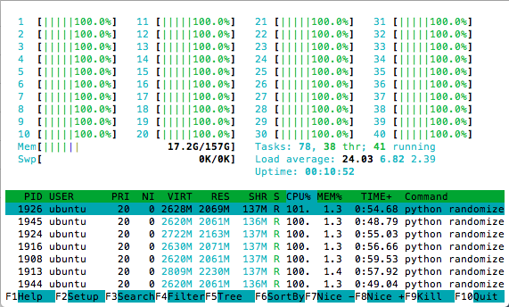
After four days of running the grid search on my four core Mac, I grew impatient and realized I would not be able to run my analysis in a reasonable amount of time. Relaunching my AWS instance became an imperative. It took me a few hours of tinkering in AWS to set up a new environment, and I was ready to continue my analysis. I set up the previous grid search to run on a 40 core instance, which I thought would allow me to generate the grid search results in a reasonable amount of time. I was wrong…
Try the lightGBM boosting algorithm.
While running the Gradient Boosting Classifier, I researched other alternatives. XGBoost and lightGBM are two popular options, with lightGBM having similar performance to XGBoost, but being 10 to 15 times faster than XGBoost.
After running the Gradient Boosting Classifier grid search for 5 hours, I stopped the computation and set up the grid search to run using the lightGBM algorithm.
The lightGBM grid search was not finished after running for 24 hours. The messages generated by the algorithm while running were indicating average f1-scores percents in the low seventies, which made me think if I wanted to let the algorithm to keep on running. Running grid searches with boosting algorithms did not seem to be generating the performance increases I was hoping for.
I stopped the grid search and took stock of what I had tried so far and of the options I had left. My first forest using boosting algorithms had not turned out to be very cost or time efficient.
Feature Engineering
After a disappointing six days of waiting, I decided it was time to try some feature design to see if we could achieve an accuracy of greater than 90% with only the hand sensor.
I calculated the pitch, roll, and norm from the x-axis, y-axis, z-axis raw accelerometer data. Also, to capture the temporal nature of the data I segmented the data into windows of various lengths and calculated the mean and variance of the signals within each window.
Using windows of size 4, 8, 16, 32 and 64 I evaluated the learning curves of trees of maximum depth 15, 20, 25, and 35. As we found earlier, trees with a depth greater than 15 were overfitting, and the accuracy of the model did not surpass 85% with any of the windows. Below is the image of the learning curves for the model when using a window of size 16.
Conclusion
Using three sensors we were able to consistently determine the activity a person was doing with accuracies greater than 90%, but we were not able to achieve this consistently when using data from 1 or 2 sensors even though we attempted some feature design. Using boosting algorithms to increase accuracy was inconclusive given that we were not able to wait until the grid search finished. A future exercise could be to try again using boosting algorithms, but we would have to design the experiment better so as not to rely so heavily on exhaustive grid searches which are extremely time-consuming.
References:
- A. Reiss and D. Stricker. Introducing a New Benchmarked Dataset for Activity Monitoring. The 16th IEEE International Symposium on Wearable Computers (ISWC), 2012.
- A. Reiss and D. Stricker. Creating and Benchmarking a New Dataset for Physical Activity Monitoring. The 5th Workshop on Affect and Behaviour Related Assistance (ABRA), 2012.